Dimensionality Reduction

차원 축소는 무엇일까? 쉽게 생각하면 그냥 말 그대로 차원을 축소한다는 말이다.

예를 들어, 내가 10차원의 features (or input data)가 있을때, 이 아이들을 모두 데리고 가기에 너무 무겁고, 많다면 이 중 정말 중요한 특성을 갖고 있는 아이들만을 뽑아내서 데리고 가겠다는 것이다.

물론, 그것이 2차원이 될 수도 혹은 5차원이 될 수도 있다.

내가 처음에 차원 축소를 접한 이유는 geophysics분야에서 seismic dataset을 해석할 때 features extraction의 관점에서 PCA를 적용하였다.

그 당시에는 PCA, ICA, 그리고 다양한 manifold learning을 고려하였지만, 여기서 내가 간과했던 점은 차원 축소 방법을 선택하기에 앞서 데이터에 대한 정확한 이해 및 그에 따른 적절한 방법론 선택이었을 거라 생각한다.

아는 만큼 보인다는 말처럼 그당시에는 정확하게 흐름을 이해하기보다는 작은 구름들이 동동 떠다니듯 ☁️ ☁️ ☁️ 이해하고 진행했던 것 같다.

어쨌든 문제를 해결하긴 하였지만, 과연 그것이 최적의 방법이었는지에 대한 의구심이 항상 내 마음 한켠에 자리잡고 있었고, 항상 마음에 걸렸었는데, 이번에 블로그 글을 작성하면서 정리하고 그 짐을 덜어 놓고자 한다.

그 식을 다 이해하기 전에는 페이지를 넘기지 말라는 Robert의 조언처럼, 이번에는 조금 느려도 정확하게 이해하고자 한다.

☾ Table of contents

☺︎ A definition of Dimensionality Reduction
☺︎ Eigenvalue and Eigenvector : 고유값, 고유벡터
☺︎ Linear Discriminant Analysis (LDA) : 선형 판별 분석
☺︎ Principal Components Analysis (PCA) : 주성분 분석
☺︎ Independent Component Analysis (ICA) : 독립 성분 분석
☺︎ Factor Analysis : 요인 분석
☺︎ Manifold learning
☺︎ Isomap
☺︎ Locally Linear Embedding (LLE)
☺︎ t-Distributed Stochastic Neighbor Embedding (t-SNE)
☺︎ Multi-dimensional Scaling (MDS)
☻ Reference

☺︎ A definition of Dimensionality Reduction

차원축소라는 것은 무엇일까?

Dimensionality reduction, or dimension reduction, is the transformation of data from a high-dimensional space into a low-dimensional space so that the low-dimensional representation retains some meaningful properties of the original data, ideally close to its intrinsic dimension. Working in high-dimensional spaces can be undesirable for many reasons; raw data are often sparse as a consequence of the curse of dimensionality, and analyzing the data is usually computationally intractable (hard to control or deal with). Dimensionality reduction is common in fields that deal with large numbers of observations and/or large numbers of variables, such as signal processing, speech recognition, neuroinformatics, and bioinformatics [1].

즉, 고차원의 데이터를 저차원의 데이터로 바꾸는 것인데, 이 저차원이 고차원일때 의미있던 정보를 대부분 cover할 수 있다는 것이다.
궁극적 목적은 정보의 손실이 거의 일어나지 않으면서 차원을 줄여서 우리가 데이터 분석, 모델 개발, 혹은 여러가지 응용분야에 사용할 수 있도록 해주는 것이다.
차원 축소의 장점으로는 훈련 속도 증가, 훈련 시간 축소, 차원의 저주 (Curse of Dimensionality) 및 과적합 (Over fitting) 방지를 통한 일반화 및 모델의 정확도, 성능 향상을 목적으로 한다.
우선 몇가지 연관성에 대하여 정리해보면,

☻ 차원의 저주와의 연관성

문제를 푸는데 있어서, 특히 머신러닝/딥러닝을 통해 모델을 학습시킬때, training set의 feature 개수가 너무 많다면 모델을 학습 속도가 느려지게 되고, 좋은 모델 즉 generalized and robust model을 얻기 힘들다[2].

The number of instances increases exponentially to achieve the same explanation ability when the number of variables increases.

☻ 과적합과의 연관성

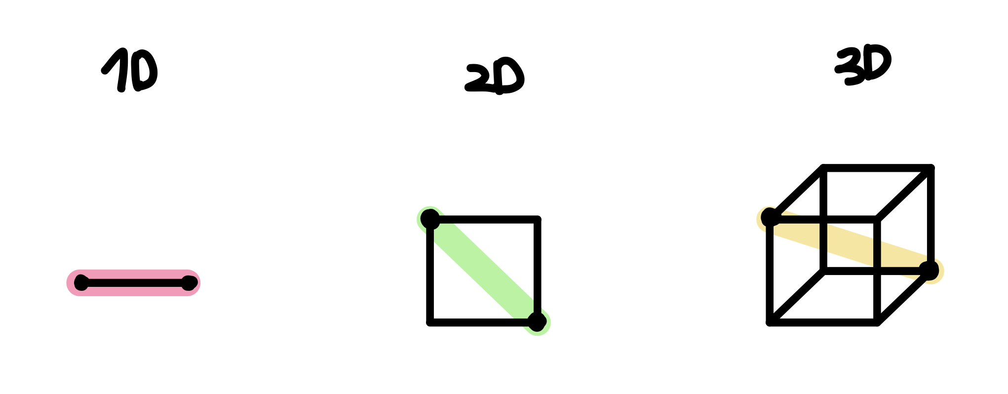
위의 그림에서 보듯, 2개의 p’t사이의 거리를 구한다고 할때, 차원이 2차원이면 0.52, 3차원이면 0.66..즉 차원이 증가할 수록 거리가 더 멀어진다. 이는 데이터 p’t 사이의 거리가 멀다.

(랜덤한 두 p’t사이의 평균 거리) 로

$\Large \sqrt{\frac{n}{6}}$

이고, n은 nth dimension). 그렇다면 모델을 학습시킨 데이터에 새로운 데이터를 추가한다면 더 멀리 떨어져있을수도 있고, 이를 위하여 예측을 위하여 더 많은 extrapolation을 해야하기 때문에 저차원보다 prediction이 불안정하게 되며 과적합 (over-fitting)의 위험성이 커진다.

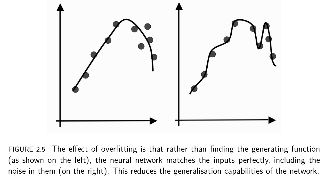
그럼 왜 overfitting을 지양하는가는 모델이 너무 복잡해지고, generalized하지 못하기 때문이다.

Ref [3]

If we train for too long, then we will overfit the data, which means that we have learnt about the noise and inaccuracies in the data as well as the actual function. Therefore, the model that we learns will be much too complicated and won’t be abble to generalise [3].

☻ 3 different ways to do dimensionality reduction [3]

Features selection: looking through the features that are available and seeing whether or not they are actually useful, i.e. correlated to the output variables.
Feature derivation: deriving new features from the old ones, generally by applying transforms to the dataset that simply change the axes (coordinate system) of the graph by moving and rotating them. The reason this performs dimensionality reduction is that it enables us to combine features and to identify which are useful and which are not.
Clustering: in order to group together similar data points, and to see whether this allows fewer features to be used.

여기서 차원의 축소에서 가장 많이 언급되는 것은 Features selection (변수 선택) 과 Feature derivation (or Features extraction, 변수 추출) 이다. Feature selection은 말 그대로 단순히 중요한 변수만을 빼내는 것이고, Feature derivation (Feature extraction)은 기존 변수 조합에서 새로운 변수 만드는 기법으로 (a) 기존 변수 가운데 일부만 활용하는 방식, (b) 모든 변수 사용 (PCA, 기존 변수를 선형 결합해서 linear combination통해 새로운 변수 만들어 냄) 이 있다.

☹︎ Features selection (변수 선택)

추가적으로 변수 선택은 feature importance test를 통해서 the most important featuers을 찾는데도 사용된다.
이는 다른 글에서 좀 더 자세히 다루도록 한다.
우선, 두가지 방법이 있는데 하나는 변수를 추가해가는 방법, 두가지는 처음에 모두 고려한 후 하나씩 빼내면서 performace가 변하지 않으면 제거하는 방법으로 아래와 같다.

Constructive (Forward selection) : decide which feature to add next. that means, it starts with none, and then iteratively and more, testing the error at each stage to see whether or not it changed at all when that features was added.
Destructive (Backward elimination) : to prune the decision tree, lopping off branches and checking whether the error changed at all[3].

☻ 차원 축소를 위한 접근 방법

차원 축소를 위한 두가지 접근법으로는

Projection (투영) : A projection is the means by which you display the coordinate system and your data on a flat surface, such as a piece of paper or a digital screen. Mathematical calculations are used to convert the coordinate system used on the curved surface of earth to one for a flat surface.
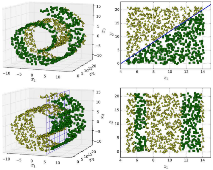
Manifold learning (매니폴드 학습) : an approach to non-linear dimensionality reduction. Algorithms for this task are based on the idea that the dimensionality of many data sets is only artificially high.

Projection (Ref [2])

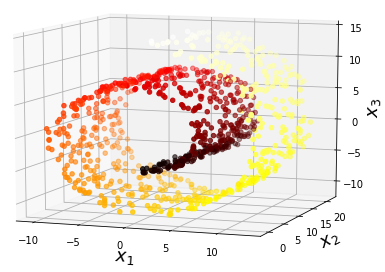
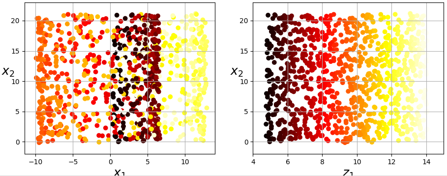
Manifold learning (Ref [2])

☺︎ Eigenvalue and Eigenvector

LDA와 PCA를 이해하는데 있어서 Eigenvalue 와 Eigenvector는 반드시 이해해야만 하는 숙명같은 존재이다.

우선, 이들의 의미를 확인하면 다음과 같다 [4].

In linear algebra, an eigenvector or characteristic vector of a linear transformation is a nonzero vector that changes at most by a scalar factor when that linear transformation is applied to it. The corresponding eigenvalue, often denoted by, is the factor by which the eigenvector is scaled. Geometrically, an eigenvector, corresponding to a real nonzero eigenvalue, points in a direction in which it is stretched by the transformation and the eigenvalue is the factor by which it is stretched. If the eigenvalue is negative, the direction is reversed. Loosely speaking, in a multidimensional vector space, the eigenvector is not rotated.

선형 변환의 eignevector (고유벡터) 는 그 선형 변환이 일어난 후에도 방향이 변하지 않는, 0이 아닌 벡터이고, eigenvalue (고유값) 은 고유 벡터의 길이가 변하는 배수를 의미한다. 기하학적으로 봤을 때, 행렬(선형변환) A의 고유벡터는 선형변환 A에 의해 방향은 보존되고 스케일(scale)만 변화되는 방향 벡터를 나타내고 고유값은 그 고유벡터의 변화되는 스케일 정도를 나타내는 값이다 [4,5].

$\Large A\mathbf{v} = \lambda \mathbf{v}$

A 는 eigenvalue, v 는 eigenvetor, 그리고 𝝺는 scalar이다.

즉, 이 과정은 scaling에 해당하는 변환이다. 따라서, 벡터를 선형변환 할대, 원점에서 멀어지는 방향으로 변환하는 scaling하는 방향을 찾는 것이 고유값 문제를 푸는 것으로 그 방향이 고유벡터의 방향이고, 그때 이동하는 거리가 고유값이 된다 [6].

여전히, 이해가 100% 이해가 되는 것은 아니다. 그럼 우리가 원하는 차원축소 (Dimensionality reduction)와의 연관성은 어떤 것일까?
LDA와 PCA에서 연관성을 기술하도록 한다.

☺︎ Linear Discriminant Analysis (LDA)

우선, LDA와 PCA는 둘다 Linear plane에 embedding을 시킨다는 공통점을 갖고 있지만, 차별성을 꼽으라면 LDA는 class (Label에 대한 정보)가 먼저 정해져야 한다는 것이다.
즉, LDA는 supervised이고, PCA는 unsupervised라고 볼 수 있다.

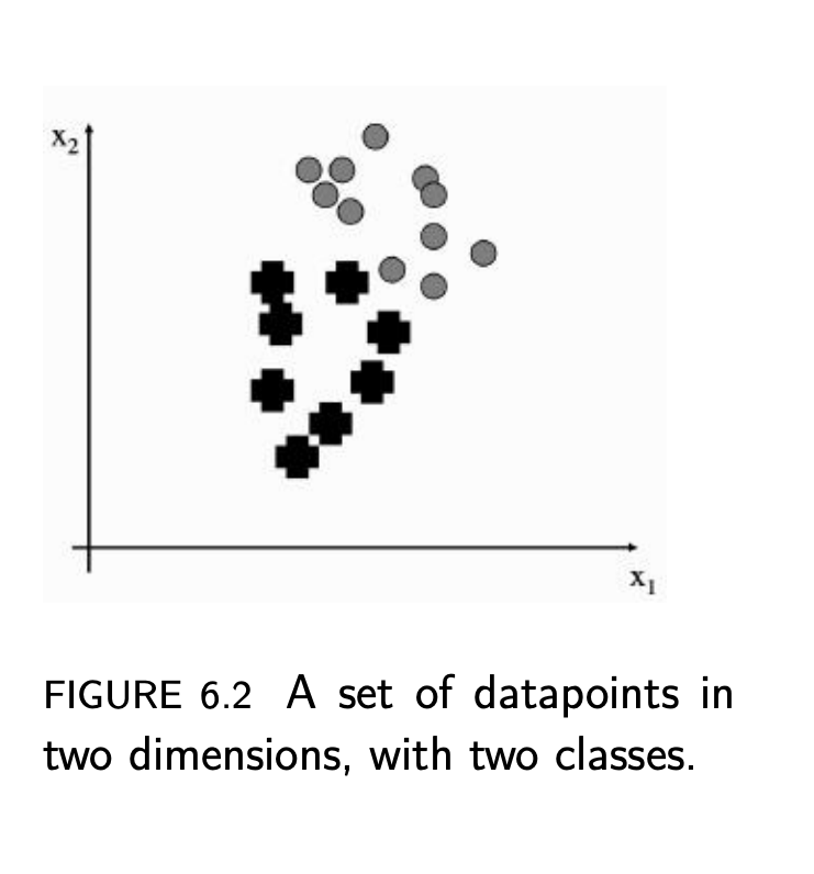
Ref [3]

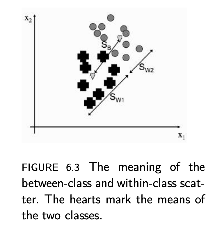
위의 그림[3]에서 처럼 두개의 classes로 구분된 데이터가 있다고 보자. 전체 데이터에서의 Mean은 𝜇, 각 class (✚과 ○)에서의 Mean을 𝜇1,𝜇2, 그리고 각 class에서의 covariance를

$\Large \sum_{j} (x_j - \mu)(x_j - \mu)^T$

라고 하자. 위의 그래프의 두 class에 표현하자면 아래와 같다.

Means

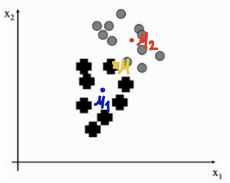
Covariance

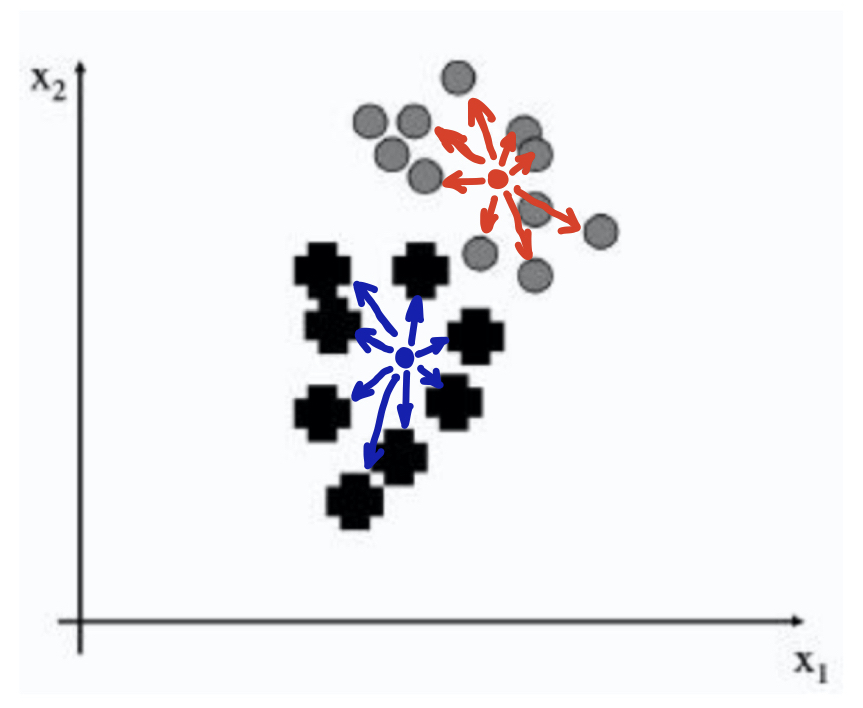
LDA의 핵심은 within-class scatter, Sw와 Between-classes scatter, SB의 비율을 최대화 (maximization) 하는 것이다. SB/Sw를 최대화함으로써 class사이는 멀어져서 잘 separation이 이뤄지고, 각 class 내부에서는 데이터끼리는 잘 모여있는 것을 의미한다.
좀 더 자세하게 살펴보면,

Ref [3]

☻ Sw, Within-class scatter

$\Large S_W = \sum_{classes c}\sum_{j\in c} p_c(x_j - \mu_c)(x_j - \mu_c)^T$

즉, 각 class 내부에서의 scatter 정도를 나타낸 값의 합으로 나타내어진다. 이 값은 작은 값을 띄어야 class에서의 데이터들이 군집되어 있다는 것을 의미하게 된다.

Covariance matrix can tell us about the scatter within a dataset, which is the amount of spread that there is within the data. The way to find this scatter is to multiply the covariance by the Pc, the probability of the class (that is the number of datapoints there are in that class divided by the total number)[3].

☻ SB, Between-classes scatter

$\Large S_B = \sum_{classes c}(\mu_c - \mu)(\mu_c - \mu)^T$

전체 데이터의 mean vector와 각 class의 mean vector사이의 거리의 제곱으로, 이 값은 큰 값을 갖아야 class끼리의 separation이 잘 이뤄진 것을 의미하게 된다.

To be able to separate the data, we also want the distance between the classes to be large. This is know as the between-classes scatter.

사실 여기서 이 SB/SW를 가능한 크게 한다는 것이 Dimensionality reduction에 대하여 어떤것도 의미하지는 않는다. 무엇을 의미하는지에 대해서 우리는 여전히 100%이해하기 힘들 것이라고 생각한다. 하지만, 차원의 수를 감소 시킬때 무언가를 한다고 말할 수는 있을 것이다. 우선, projection에 대해서 생각해보자.

앞에서 차원 축소를 위한 두가지 접근법 중 하나가 Projection (투영)이라고 했다.

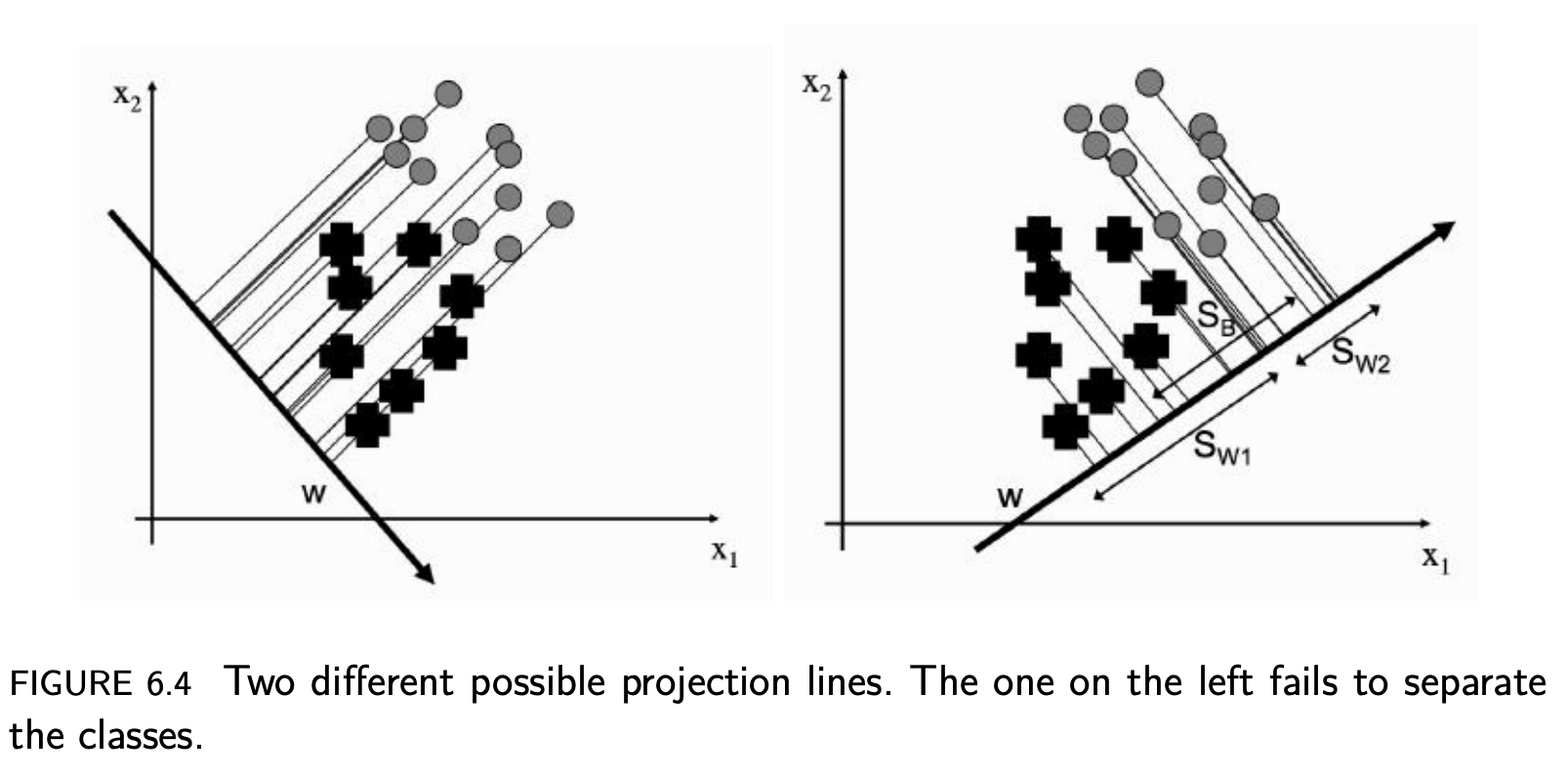
Ref [3]

우리가 아까부터 봐왔던 데이터를 하나의 linear line에 projection시킨다고 할 때, 위의 그림처럼 Vector, w 에 따라서 다르게 나타난다.
우선, projection of the data can be written as

$\Large z = \mathbf{w}^T \cdot \mathbf{x}$

여기서, x 는 datapoint. 이 것은 우리에게 scalar값을 주는데, 이 scalar가 the distance along the w vector 이다.

Projection
To see remember that the equation, we write above, is the sum of the vectors multiplied together element-wise, and is equal to the size of w times the size of x times the cosine of the angle between them. We can make the size of w be 1, so that we don’t have to worry about it, and all that is then described is the amount of x that lies along w. So we can compute the projection of our data along w for every point, and we will have projected our data onto a straight line.

자! 이제 within-class scatter과 between-class scatter에 간단한 작업을 통해 왜 SB/Sw의 최대화 (maximization)와 dimensionality reduction이 연관되어 있는지 확인하려 한다.

$\Large \sum_{classes c}\sum_{j\in c} p_c (\mathbf{w}^T \cdot (x_j - \mu_c))(\mathbf{w}^T \cdot (x_j - \mu_c))^T = \mathbf{w}^T S_w \mathbf{w}$

$\Large \sum_{classes c}\mathbf{w}^T(\mu_c - \mu)(\mu_c - \mu)^T\mathbf{w} = \mathbf{w}^T S_B \mathbf{w}$

이 두 값의 비율은 Objective function, J(w)로

$\Large J(\mathbf{w}) = \frac{\mathbf{w}^T S_B \mathbf{w}}{\mathbf{w}^T S_w \mathbf{w}} \Uparrow$

In order to find the maximum value of this with respect to w, we differentiate it and set the derivative equal to 0 :

$\Large \frac{S_B\mathbf{w}(\mathbf{w}^T S_W \mathbf{w})-S_W\mathbf{w}(\mathbf{w}^T S_B \mathbf{w})}{(\mathbf{w}^T S_W \mathbf{w})^2} = 0$

여기서 Projection vector, w를 풀면 된다.

$\Large S_W \mathbf{w} = \frac{\mathbf{w}^T S_W \mathbf{w}}{\mathbf{w}^T S_B \mathbf{w}} S_B \mathbf{w}$

여기서 right hand side를 조금만 수정해보면 [7] 괄호 안의 값은 scalar가 되고, 이것을 다시 쓰면 다음과 같다.

$\Large S_W \mathbf{w} = \lambda S_B \mathbf{w}$

$\Large S_B^{-1} S_W \mathbf{w} = \lambda \mathbf{w}$

이 식은 Eigenvalue, Eigenvector식과 유사하다 (아래 식 참고)

$\Large A\mathbf{v} = \lambda \mathbf{v}$

A 는 eigenvalue, v 는 eigenvetor, 그리고 𝝺는 scalar이다.

따라서, Known values인 Sw, SB 그리고 scalar값인 𝝺와 Eigenvalue decomposition통해서 새로운 축 w를 구할 수 있다.

☺︎ Principal Components Analysis (PCA)

이제 unsupervised 인 PCA를 보도록 하자.
우선, PCA는 차원축소에서 가장 많이 쓰이는 방법이다. 이는 꼭 차원 축소 뿐만 아니라, 데이터 압축, feature 추출, 데이터 시각화등에도 널리 사용되고 있다 [7].

Principal Component Analysis, or PCA, is a techinique that is widely used for applications such as dimensionality reduction, lossy data compression, feature extraction, and data visualization (Jolliffe,200).

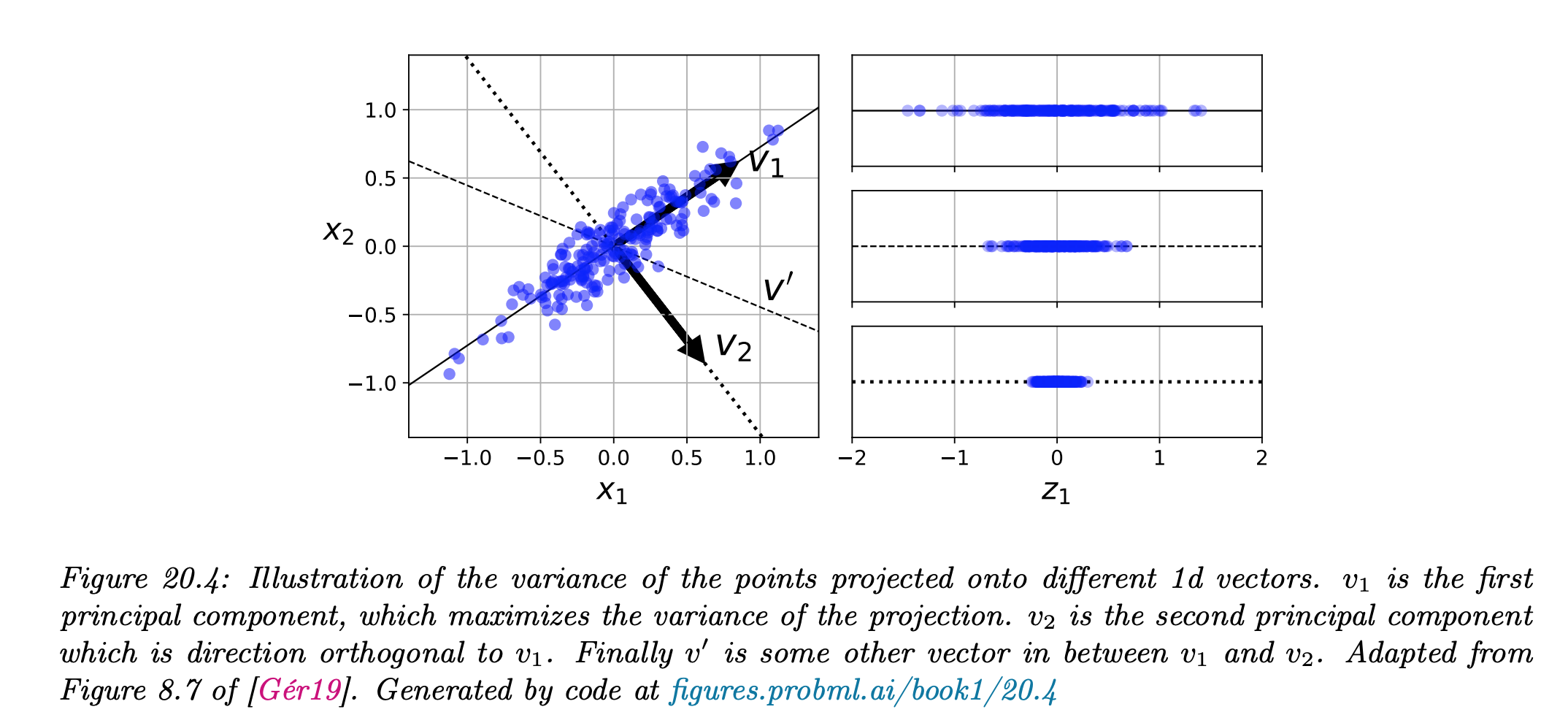
그럼, PCA는 무엇을 하는 것일까? 간단히 말해 데이터의 공분산이 큰 방향을 찾는 것이다.

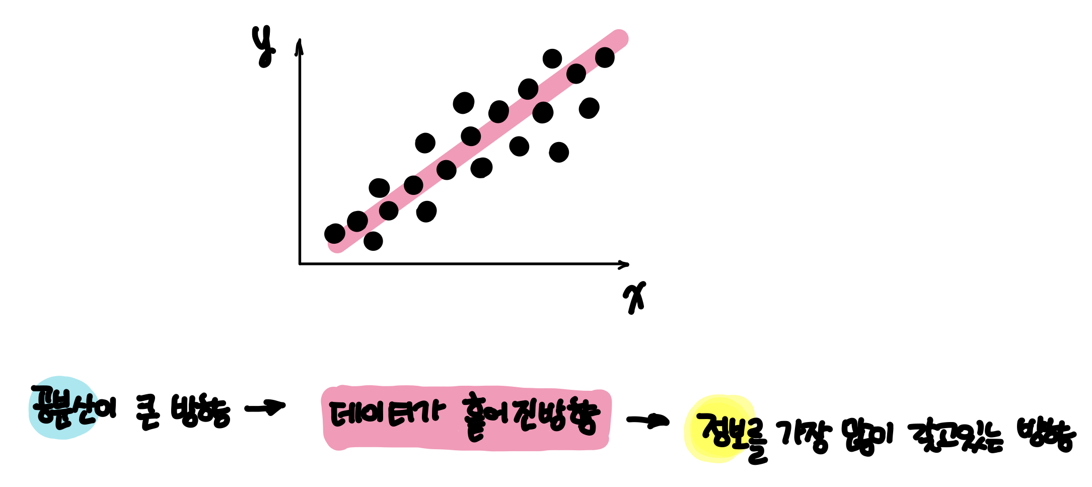
왜? 왜 공분산이 큰방향을 찾는걸까?
그 해답은 위의 그림처럼 데이터가 흩어진 방향으로 차원 축소를 한다면 가장 많은 정보를 갖게 되고 역으로 가장 적은 정보 손실이 이뤄진다는 말이다. 이것이 우리가 차원축소에서 궁극적으로 추구하는 방향이라 할 수 있다.

좀 더 자세하게 살펴보자.

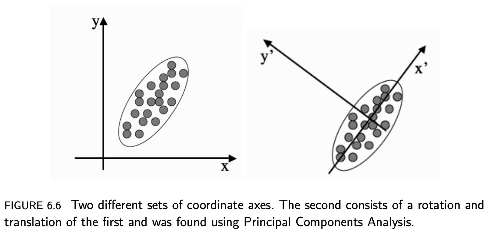
Ref [3]

The idea of a principal component is that it is a direction in the data with the largest variation. The algorithm first centres the data by subtracting off the mean, and then chooses the direction with the largest variation and places an axis in that direction, and then looks at the variation that remains and finds another axis that is orthogonal to the first and covers as much of the remaining variation as possible. It then iterates this until it has run out of possible axes. The end result is that all the variation is along the axes of the coordinate set, and so the covariance matrix is diagonal—each new variable is uncorrelated with every variable except itself. Some of the axes that are found last have very little variation, and so they can be removed without affecting the variability in the data [3].

즉, the lagest variation을 갖는 직교 성분 축을 찾고, 반대로 little variation, 즉 data information이 적은 것은 제거한다는 것이다. Principal component (주성분)은 가장 분산이 큰 방향이기 때문에 주성분에 투영하여 바꾼 데이터는 원본이 가지고 있는 특성을 잘 나타내고 있을 것이다.

PCA에 대한 Kevin Murphy의 설명은 다음과 같다 [9].

The basic idea is to find a linear and orthogonal projection of the high dimensional data x ∈ R^{D} to a low dimensional subspace z ∈ R^{L}, such that the low dimensional representation is a “good approximation” to the original data, in the following sense: if we project or encode x to get z = w^{T}x, and then unproject or decode z to get x’ = wz, then we want x’ to be close to x in l2 distance. In particular, we can define the following reconstruction error or distortion.

순차적인 과정은 다음과 같다.

데이터 X에서 평균을 구하고, 그 평균에 좌표축을 가져감.
공분산 행렬 계산
이에 대한 고유값과 고유벡터 구함
고유벡터 방향으로 데이터를 표현하면, 가장 큰 분산을 가지는 데이터를 나타낼 수 있음

좀 더 디테일한 관점에서 바라본다면 [7], 데이터 X를 w라는 새로운 축에 projection (투영)시켜, z라는 새로운 행렬을 구합니다.

$\Large \mathbf{z} = \mathbf{w}^{T} \mathbf{X}$

차원 축소의 원래 목표는 데이터의 정보를 최대한 보존 = 데이터 X의 분산의 최대화이므로 결국 z의 분산도 최대화가 되야 한다. 이를 식으로 나타내면

$\Large \begin{matrix} \mathbf{max} \left{ Var (\mathbf{z}) \right} &=& \mathbf{max} \left{ Var(\mathbf{w}^{T} \mathbf{X}) \right}\ &=& \mathbf{max} \left{ \mathbf{w}^{T} Var(\mathbf{X})\mathbf{w}\right} &=& \mathbf{max} \left{ \mathbf{w}^{T} \mathsf{\Sigma} \mathbf{w}\right} \end{matrix}$

여기서 w 의 크기를 크게 하는 것만으로도 z의 분산을 높일수 있으므로 제약식을 준다.

$\Large \parallel \mathbf{w} \parallel = \mathbf{w}^{T} \mathbf{w} = 1$

이를 라그랑지안 문제로 변형하면,

$\Large L = \mathbf{w}^{T} \mathsf{\Sigma} \mathbf{w} - \lambda ( \mathbf{w}^{T} \mathbf{w} - 1)$

미분을 해서 최대값을 구하면,

$\Large \frac{\partial L}{\partial \mathsf{w}} = \mathsf{\Sigma} \mathbf{w} - \lambda \mathbf{w} = 0$

$\Large ({\Sigma} - \lambda) \mathbf{w} = 0$

w는 데이터 X의 공분산 행렬인 ∑에 대한 eigenvector (고유벡터)이며, 이를 Principal component (주성분)이라고 한다.

좀 더 디테일한 부분은 추가적 이해를 한 후 작성하고자 한다.

Ref [9] 관심있다면, 유명한 Youtube를 추천한다. 개인적으로 intro song은 무척 맘에 든다 :)

https://www.youtube.com/watch?v=HMOI_lkzW08&t=64s

☻ Kernel PCA

차원 축소를 위한 복잡한 비선형 투형을 수행하기 위한 기법으로, 이 또한 unsupervised learning이므로 좋은 커널과 하이퍼파라미터 선택을 위한 명확한 성능 측정 기준은 없다 [1]. 좀 더 자세한 내용은 추후 업데이트 예정이다

☻ Reference

https://en.wikipedia.org/wiki/Dimensionality_reduction
[book, 개인 소장] Hands-on Machine laerning with Scikit-Learn Keras & TensorFlow : 핸즈온 머신러닝 2판
[book, 개인 소장] Machine Learning: An Algorithmic Perspective by Stephen Marsland
https://en.wikipedia.org/wiki/Eigenvalues_and_eigenvectors
[블로그] https://darkpgmr.tistory.com/105
[블로그] https://m.blog.naver.com/PostView.naver?isHttpsRedirect=true&blogId=je1206&logNo=220818602286
[Github blog] https://ratsgo.github.io/machine%20learning/2017/03/21/LDA/
[book, 개인 소장] Pattern Recognition and Machine Learning
[book, 개인 소장] Machine Learning: A Probabilistic Perspective

Written on May 5, 2022