Linear Regression
[코드리뷰 | 개념] Linear Regression
This article is based on Medium Blog titled ‘Introduction to Linear Regression in Python’[1].
이 블로그 글은 Medium Blog titled by ‘Introduction to Linear Regression in Python’[1]과 Mathematics for Machine Learning (MML)책[6]을 reference로 해서 작성하였습니다.
What the Linear Regression is…
☾ Table of contents
☺︎ Linear Regression
- y_hat (predicted value) vs y (ground truth)?
☺︎ Linear regression w/ the OLS method
- Dataset
- the OLS method
☺︎ Linear regression w/ statsmodels
- Dataset
- statsmodels’ ols function
☺︎ Linear regression w/ scikit-learn
☻ Reference
☺︎ Linear Regression (선형회귀)
선형 회귀를 다루기 전에 회귀 (regression)의 개념을 확인해보자.
회귀 (regression)의 사전적 의미를 확인하면 아래와 같다 [2,3].
◦ Regression
  1. a return to a former or less developed state.
  2. `STATISTICS` a measure of the relation between the mean value of one variable (e.g. output) and corresponding values of other variables (e.g. time and cost).

◦ 회귀
  1. 한 바퀴 돌아 제자리로 돌아오거나 돌아감.
  2. 하나의 종속 변수와 두 개 이상의 독립 변수 사이에 나타나는 관계를 최소 제곱법으로 추정하는 방법.
이에 대해서 wikipedia에서 기술한 definition을 확인하면 다음과 같다 [4].
In statistical modeling, regression analysis is a set of statistical processes for estimating the relationships between a dependent variable (often called the ‘outcome’ or ‘response’ variable, or a ‘label’ in machine learning parlance) and one or more independent variables (often called ‘predictors’, ‘covariates’, ‘explanatory variables’ or ‘features’). The most common form of regression analysis is linear regression, in which one finds the line (or a more complex linear combination) that most closely fits the data according to a specific mathematical criterion.
즉, 정리해보면 독립변수 (x) 와 종속변수 (y) 의 관계를 찾아내는 것이 회귀이다. 이 중 가장 일반적이고 흔한 형태가 선형회귀 (Linear regression)인데, 이는 특정 수학적인 기준에 따라서 데이터가 가장 근접하고 잘 맞는 선을 찾는 것이라고 한다 (직역을 하다보니 해석이 좀 이상한 부분은 양해 부탁드려요 🙏🏻)
좀 더 간단하게 식을 통해 회귀를 살펴보면 다음과 같다.
여기서 독립변수는 x로 input/predictor value이고, 종속변수 y는 output/label variable (ground truth), 그리고 𝜀 은 random noise로 우리가 완벽하게 예측하는 것은 불가능에 가깝다. 따라서 이 식을 조금 정리하면 다음과 같고,
이를 조금만 더 정리해보면 아래와 같이 y와 y_hat의 식으로 나타낼 수 있다.
여기서 우리의 관심사는 실제 데이터인 y에 가장 근접한 y_hat을 찾아내는 것이다. 즉, 𝜟y = y - y_hat을 작게 만드는 것으로, 이를 위해서는 y_hat에 대한 함수인 f(x), 특히 이 함수의 paramters인 𝛼와 𝛽 의 최적값을 구하는 것이 우리가 앞으로 하고자 하는 바이다.
☻ y_hat (predicted value) vs y (ground truth)?
앞으로 나아가기에 앞서 y_hat은 무엇일까? y는 실제 데이터라고 했는데, y_hat은 과연 무엇일까?
이것을 이해하기에는 이전 블로그 글인 Data톺아보기의 ‘☻ Find the hidden data ‘부분을 읽어보길 바란다.
사실 자연에서 일어나는 것을 포함한 우리 주변의 모든 현상을 간단한 식으로 나타내기는 쉽지 않다 [5].
우리가 많이 다루는 수학적/물리학적 이론이나 식들은 실제 현상을 constraints, assumption, and conditions등을 고려해서 가장 근사하게 나타낸 것 인다. 왜냐하면 현상이란 우리가 생각하는 것보다 무척 복잡하기때문에 우리가 정의하고자 하는 어떠한 모델, 식, 방법론으로 완벽하게 나타내기 힘들며, 이는 (극단적인 표현으로 말하자면) 오직 신만이 정확하게 구현할 수 있다고 생각한다.
따라서 수많은 수학, 물리 혹은 다른 모든 도메인에서 문제를 풀 때 exact solution (참값)이 아닌 approximate solution (근사값)을 구한다. 이때, 중요한 것은 exact solution과 approximation solution의 차이를 최소로 하는 최적화된 값을 구하는 것이 중요하다.
이런 관점에서 본다면 Linear regression에서 중요한 부분은 predicted value (이해를 돕기위해 approximate solution과 같은 개념으로 이해하면 좋을 것 같다)인 y_hat과 실제 데이터인 y의 차인 𝜟y = y - y_hat을 가장 작게하는 parameters인 𝛼와 𝛽 을 구하는 것이다.
데이터 관점에서 이를 이해하고자 한다면 아래와 같다 [6].
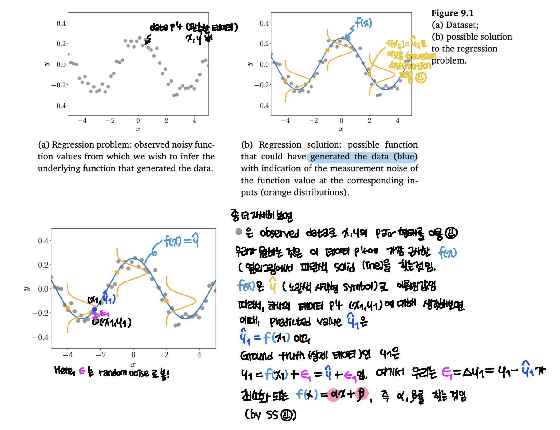
In regression, we aim to find a function f that maps input x ∈ ℝ^{D} to correspnding function value f(x) ∈ ℝ. We assume we are given a set of training input x and correponding noisy observation y = f(x) + 𝜀, where 𝜀 is an i.i.d. random variable that describes measurement/observation noise and potentially unmodeled processes.
좀 더 자세한 이해를 위해 그림을 확인해보자 [6].
(아래 schematic은 MML의 Figure 9.1에 한글로 내용을 추가해서 작성한 것 입니다.)
자, 이제 Medium blog [1]에 나와있는 코드를 구현함으로써 좀 더 자세하게 이해해보도록 하자.
☺︎ Linear regression w/ the Ordinary Least Squares (OLS) method
실제 데이터를 통하여 문제를 풀때는 Scikit learn의 LinearRegression function을 사용한다. 하지만, 그 전에 mechanism을 잘 이해하는 것이 무척이나 중요하므로 우리는 실제 Linear regression을 random data와 the Ordinary Least Squares (OLS) method로 구현하고, 𝛼와 𝛽 를 구하는 작업을 수행하고자 한다.
(자세한 코드 및 설명은 🌈Code: Jupyter notebook를 참고하세요.)
☻ Dataset
여기서 고려한 데이터는 총 100개의 random 데이터로 mean = 1.5, stddev = 2.5값을 있다.
(base) print(np.mean(x),np.mean(y))
=========================================
 check statistical values
-----------------------------------------
x_mean: 1.6495200388362121
y_mean: 2.5358624970247825
=========================================
☻ the OLS method
Objective of the least squares (OLS) method 을 통해 𝛼와 𝛽를 구하면 아래와 같다 [1].
where X^bar and Y^bar are the mean values of X and Y.
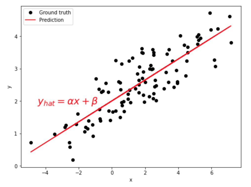
데이터 분포를 시각화하면 아래와 같다. black circle 이 실제 ground truth data p’t 이고, red solid line이 predicted value로 이뤄진 function이다.
(base) print('alpha=',alpha,'beta=',beta)
=========================================
alpha = 0.3229396867092763
beta = 2.0031670124623426
=========================================
따라서, 여기서 구한 최적의 함수는 f(x) = 0.32 x + 2 이다.
이제는 두개의 python modules인 statsmodels 과 scikit-learn을 이용하도록 한다 [1].
◦ statsmodels — a module that provides classes and functions for the estimation of many different statistical models, as well as for conducting statistical tests, and statistical data exploration.
◦ scikit-learn — a module that provides simple and efficient tools for data mining and data analysis.
☺︎ Linear regression w/ statsmodels
사용하고자 하는 데이터는 advertising data로, kaggle에서 다운 받을 수 있다 [7].
(자세한 코드 및 설명은 🌈Code: Jupyter notebook를 참고하세요.)
☻ Dataset
데이터는 총 200개의 row와 4개의 column으로 구성되어 있다.
(base) print(advert.shape)
(base) print(advert.describe())
(base) print(advert.head())
=========================================
total size :  (200, 4)
-----------------------------------------
               TV       Radio   Newspaper       Sales
count  200.000000  200.000000  200.000000  200.000000
mean   147.042500   23.264000   30.554000   15.130500
std     85.854236   14.846809   21.778621    5.283892
min      0.700000    0.000000    0.300000    1.600000
25%     74.375000    9.975000   12.750000   11.000000
50%    149.750000   22.900000   25.750000   16.000000
75%    218.825000   36.525000   45.100000   19.050000
max    296.400000   49.600000  114.000000   27.000000
=========================================
      TV  Radio  Newspaper  Sales
0  230.1   37.8       69.2   22.1
1   44.5   39.3       45.1   10.4
2   17.2   45.9       69.3   12.0
3  151.5   41.3       58.5   16.5
4  180.8   10.8       58.4   17.9
=========================================
☻ statsmodels’ ols function
statsmodels을 이용해서 구하면 아래와 같다 [8].
statsmodels.formula.api: A convenience interface for specifying models using formula strings and DataFrames. This API directly exposes the from_formula class method of models that support the formula API. Canonically imported using import statsmodels.formula.api as smf
여기서는 x는 TV dataset을 y는 Sales만 고려하였다.
(base) print(model.params)
=========================================
Intercept    6.974821
TV           0.055465
dtype: float64
=========================================
여기서 Intercept가 𝛽이고, TV가 𝛼이다. 식으로 나타내면 sale = 0.05x + 6.97이다.
데이터 분포를 시각화하면 아래와 같다. black circle 이 실제 ground truth data p’t 이고, red solid line이 predicted value로 이뤄진 function이다.
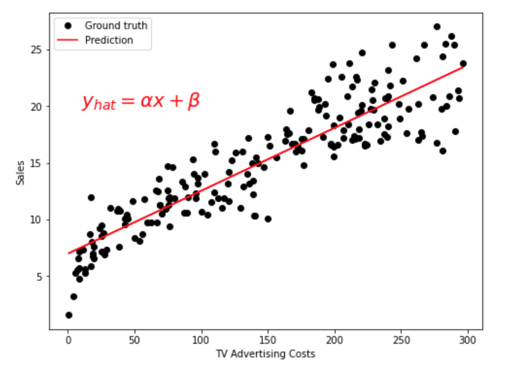
이를 통해서 TV 광고를 많이 할수록 많이 팔린다는 것을 확인 할 수 있었다.
☺︎ Linear regression w/ scikit-learn
앞에서는 1개의 독립변수 (univariable)을 이용했다면, 여기서는 여러개의 독립변수 (multivariable)을 고려해서 multiple Linear regression을 만들도록 한다.
univariable/multivariable과 univariate/multivariate에 대하여 궁금하다면 기존 작성한 Multivariate (다변량) vs Multivariable (다변수)란?를 참고하세요[5].
(자세한 코드 및 설명은 🌈Code: Jupyter notebook를 참고하세요.)
여기서는 multivariable를 고려하였으므로, 독립변수 x가 여래개이며 식은 아래와 같이 나타낼 수 있다.
데이터는 위에서 사용한 advertising data와 동일하며, x1인 TV와 x2인 Radio, y는 Sales을 고려하였다.
(base) print(f'alpha = {model.coef_}')
(base) print(f'beta = {model.intercept_}')
=========================================
alpha = [0.05444896 0.10717457]
beta = 4.63087946409777
=========================================
여기서 구한 multiple linear regression model에 우리가 갖고 있는 TV와 Radio 데이터 (혹은 새로운 데이터)를 고려해서 sales을 예측할수 있다.
본 블로그 글에서는 MML에서 배운 내용을 기반으로 Linear regression의 개념을 이용하고 Medium blog에 있는 Introduction to Linear Regression 을 직접 모사함으로써 이론과 실습을 모두 해보았다.
후에는 실제 복잡하고 다양한 데이터에 적용시켜볼 예정이다.
☻ Reference
- Medium: Introduction to Linear Regression in Python
- [Oxford Languages]
- 네이버 국어/영어사전
- wikipedia: Regression analysis
- blog: ABB
- Book: Mathematics for Machine Learning
- kaggle : Advertising Dataset
- statsmodels, API Reference
☻ image sources
Thanks for reading. Hope to see you again :o)